In this lecture, we still talk about sorting and we want to ask “How fast can we sort?”. Let’s review the running time of previous learned Algorithms, the Heapsort and Merge Sort can achieve ${ O(n \lg n) }$ in the worst case. Randomized Quicksort can run in ${ O(n \lg n) }$ time on average. And Insetion Sort is ${ O(n^2) }$. All these Algortihms run no faster than ${ O(n \lg n) }$.

So can we do better?

No but Yes!. In fact, it depends on what kinds of manipulation are allowed. The Algorithms mentioned before have a common property: the sorted order they determine is based only on comparisons between the input elements. So, such sorting algorithms are called comparison sort. In this sense, the Anwser is No! We gonna prove that any comparison sort cannot run faster than ${ O(n \lg n) }$ in the worst case.

From another way, if we use other oprations more than “Comparison”, we can get some sorting algorithms faster than ${ O(n \lg n) }$. In this lecture, we will introduce Counting sort and Radix sort.

Lower bounds for Comparison sorts

In a compasison sort, we can only use comparisons to gain the order information about input sequence ${ \left< a_1,a_2,\cdots, a_n \right> }$. In this section, we assume the all elements in array are distinct. Here we introduce decision tree.

Decision tree model

We can view the comparison sorts in terms of decision tree. A decision tree is a full binary tree that represents the comparsion between elements that are performed by a particular sorting algorithm operating on an input of a given size. In another words, for a given size of input, we can use decision tree to represent the algorithm, in which we only record each comparison in node, and the different result will lead to different child nodes.

Let’s take an example to get some intuition. Suppose we want to sort three elements ${ \left< a_1, a_2, a_3\right> }$. Here is the solution of insertion sort

first move to second element ${ a_2 }$, and then compare ${a_2}$ to ${ a_1 }$. If ${ a_2 \geq a_1 }$, then we move to ${ a_3 }$, compare ${ a_2, a_3 }$ … consider all the situation, we can get following decision tree

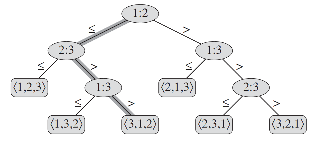
The decision tree for insertion sort operating on three elements.

Definition of Decision tree

In general, for a given list ${ \left< a_1,a_2,\cdots, a_n \right> }$

• Each internal node (non-leaf node) has a lable “${ i:j }$”, ${ i, j \in { 1,2,\cdots, n } }$, which means we compare ${ a_i , a_j }$

• Left subtree gives the subsequent comparisons if ${ a_i \leq a_j }$

• Right subtree gives the subsequent comparisons if ${ a_i > a_j }$

• Each leaf node gives a permutation ${ \left< \pi(1), \pi(2), \cdots, \pi(n) \right> }$ such that ${ a_{\pi(1)} \leq a_{\pi(2)} < \cdots < a_{\pi(n)} }$

Decision tree model comparison sorts

• One tree for each input size ${ n }$

• View algorithms as splitting whenever it makes a comparision.

• Tree lists comparisons along all posible instruction traces.

The number of leaves is ${ n! }$, which is all the possible permutation of ${ n }$ elements.

Lower bounds

• The runing time of one certain case raltes to the number of comparision, which equals to the length of the path from root to the leaf.

• The worst-case runing time is the height of the tree.

Theorem Any comparison sort algorithm requires ${ \Omega(n \lg n) }$ comparisons in the worst case.

Proof. The number of leaves is at least ${ n! }$. We denote the tree of the tree as ${ h }$. So, we have to guarantee

Corollary Heapsort and merge sort are asymptotically optimal comparison sorts.

Proof. It’s easy to check from above Theorem.

Randomized algorithm

The above conclusions apply to “Deterministic algorithms” (like Heapsort, Insertion sort). What a Deterministic algorithm does is completely determine at each step! But, for a randomized algorithm, it will depend on some Randomized factors. Reviewing the “Definition of Decision Tree”, we assume only one tree for each input size ${ n }$. Therefore, for randomized algortihms, we actually get a series of trees (the probability distribution of trees). But the lower bound is still applies to it, though. Because, no matter what tree we get, the above conclusion applies to every tree.

Counting sort

Counting sort assumes that each of the ${ n }$ input elements ${ A[i] \in {0,2, \cdots , k } }$. The idea of Counting sort is counting how many elements less than each element ${ x }$, and determining the postion of ${ x }$. Like there are ${ 17 }$ elements less than ${ x }$, ${ x }$ will be put on the ${ 18^{\text{th}} }$ position in output array.

In the pseudocode of Counting sort, we use ${ A[1..n] }$ to represent input array, ${ B[1..n] }$ to denote output array, and ${ C[1..k] }$ as temporary auxiliary storage.

1
2
3
4
5
6
7
8
9
10
11
COUNTING-SORT(A,B,K)
let C[0..k] be a new array
for i = 0 to k
    C[i] = 0
for j = 1 to n
    C[A[j]] =  C[A[j]] + 1 // C[i] now counts the number i in array A.
for i = 1 to k
    C[i] = C[i] + C[i-1] // C[i] now stores the number of elements which are not greater than i. 
for j = n downto 1
    B[C[A[j]]] = A[j] //Input A[j] to B, its position is determined by C[A[j]]
    C[A[j]] = C[A[j]] - 1 // Because element A[j] has been put into B, and the conuting number minus 1.

For second loop, we use the ${ i^{\text{th}} }$ postion of ${ C }$ to count the number of elements which equals to ${ i }$, that is ${ C[i] = \vert {e = i, e \in A[1..n]}\vert }$. For third loop, array ${ C[i] }$ holds the number less than or equal to ${ i }$, ${ C[i] = \vert {e \leq i, e \in A[1..n]}\vert }$ which also represents the last position of element that equals to ${ i }$. The last loop puts all the elements of ${ A }$ to correct position. We iterate ${ A }$ from the end, each time when we pick up ${ A[j] }$, we can get the position from ${ C[A[j]] }$ and update ${ C[i] }$.

From the pseudocode, we can easily get the runing time of Algorithm is ${ \Theta(k+n) }$. If ${ k = O(n) }$, we will get a linear algorithm.

Stability of Counting Sort

An important property of counting sort is that it is stable: numbers with the same value appear in the output array in the same order as they do in the input array. Because COUNTING-SORT iterates array ${ A }$ in reverse order, and in each time places the elements with same value from back to front. So, these elements with same value keep the origin order.

Counting sort’s stability is important, because counting sort is often used as a subroutine in radix sort.

Stability of Comparison Sorts

Let’s talking about the stability of these Comparison Sorts.

1. Insertion Sort

Consider two elements with index ${ i,j }$ and ${ i < j }$ have same value. Insertion sort scan the array from first element to the end. When we iterate at ${ j^{\text{th}} }$ postion, element ${ i }$ will first be arranged in an appropriate postion such that the first ${ j-1 }$ elements have been sorted. In each loop, we will scan the array from current postion in reverse order. And, we will push the elements before ${ j^{\text{th}} }$ postion to next, when its value is greater than ${ A[j] }$. So, when compare ${ A[i],A[j] }$, move will not happen due to their same value. That means, Insertion Sort keeps the same order with origin array.

2. Merge Sort

Consider two elements with index ${ i,j }$ and ${ i < j }$ have same value. No matter when Merge Sort merges subarray with ${ A[i] }$ and subarray with ${ A[j] }$, subarray with ${ A[i] }$ will become the left array and subarray with ${ A[j] }$ will become the right array. In Merge arrays in each time, but for the situation that two elements have same value, Merge Sort will choose the left one. Therefore, Merge Sort is also stable!

3. HeapSort

It’s not a stable sort. We can give an example ${ A = \left< 2, 1a, 1b\right> }$. Here we use ${ a,b }$ to denote the order of these two elements with value as ${ 1 }$. First time, heapsort will pick up ${ 2 }$ to the end. At that time, ${ [1a, 1b] }$ still maintain the heap property, so heapsort will exchange the first element ${ 1a }$ to ${ 1b }$. In the end, we get ${ 1b, 1a, 2 }$.

4. QuickSort

It’s not a stable sort. We can give an example ${ A = \left<1a, 1b, 2\right> }$. First, we choose ${ 1a }$ as pivot, so we will partition the array, so we get ${ 1b, 1a, 2 }$. In the end, we will find the output array is not the same order with origin one.

Radix sort

Radix sort is the algorithm used by the card-sorting machines. For decimal digits, each column uses only 10 places. A ${ d }$-digit number would then occupy a field of d columns. Since the card sorter can look at only one column at a time, the problem of sorting n cards on a d-digit number requires a sorting algorithm.

Intuitively, you might sort numbers on their most significant digit, put the cards with same value into a bin. Then we sort each of the resulting bins recursively. Unfortunately, since the cards in 9 of the 10 bins must be put aside to sort each of the bins, this procedure generates many intermediate piles of cards that you would have to keep track of. With the number of digit growing up, we need more and more bins. That’s a horrible thing.

Counterintuitively, we need sorted from the least significant digit first! But here we must use a kind of Stable Sorting Algorithms.

Correctness

We induct on the digit position ${ t }$. Assume that the ${ t-1 }$ digits beyond ${ t }$ have sorted. Now, we sort the ${ t }$ digit. There are two cases

1. If two elements have same ${ t^{\text{th}} }$ digit. By the Stability we know they keep in the same order. So, they are in sorted order by induction hypothesis.

2. If the two elements have differential ${ t^{\text{th}} }$ digit. Due to the correctness of Sorting Algorithms, we will sort them in right order.

Hence, we prove the correctness.

Runing time

For each round, we use Counting Sort, which takes ${ O(n+k) }$ in each digit. Suppose we have ${ n }$ integers with ${ b }$ bits long (range from ${ 0 }$ to ${ 2^b -1 }$). But, here we don’t have to use split these numbers as digits. We try to find out the best way. So, we split these binary integer into ${ b/r }$ “digits” each ${ r }$ bits long(${ k = 2^r }$). So, the number of rounds is ${ b/r }$. Hence, we can get the runing time ${ T(n) }$

Choose ${ r }$ to minimize ${ T(n) }$, we can denote ${ f(r) = \frac{b}{r}\cdot (n+2^r) }$. In this function, ${ \frac{b}{r}\cdot n }$ wants ${ r }$ big and ${ \frac{b}{r}\cdot 2^r }$ wants ${ r }$ small, in which ${ 2^r }$ dominates this formula. So, we don’t want ${ 2^r \gg n }$, that implies we can choose ${ r }$ subject to ${ n = 2^r \Rightarrow r = \lg n}$. Therefore, ${ T(n) = O(bn/ \lg n) }$.