Today, we will introduce a very interesting Algorithm, called “Quicksort”, which was invented by Tony Hoare in 1962.

• It’s also a Divide-and-Conquer Algorithm.

• The array will be sorted “in place”. (That means Quicksort doesn’t need extra array like Mergesort.) Therefore, it’s fairly efficient in its use of storage.

• Very pratical (with tuning)

Idea of Quicksort

1. “Divide”: Partition array into 2 subarray arond pivot ${ x }$, such that

1. “Conquer”: Recursively sort the two subarray.

2. “Combine”: Trivial

So, the key point is te “Divide” Step. We can treat the Quicksort as recursive partitioning, and the Mergesort is recursive merging. Here, we can give a linear time ${ \Theta(n) }$ partiioning subroutine and give its pseoudocode

1
2
3
4
5
6
7
8
9
Partitioning(A,p,q): // treat A[p···q]
    x = A[p] // pivot is A[q]
    i = p // set index
    For j = p+1 to q
        if A[j] <= x 
            i = i + 1
            exchange A[i] with A[j]
    exchange A[p] with A[i]
    return i

Correctness of Quicksort

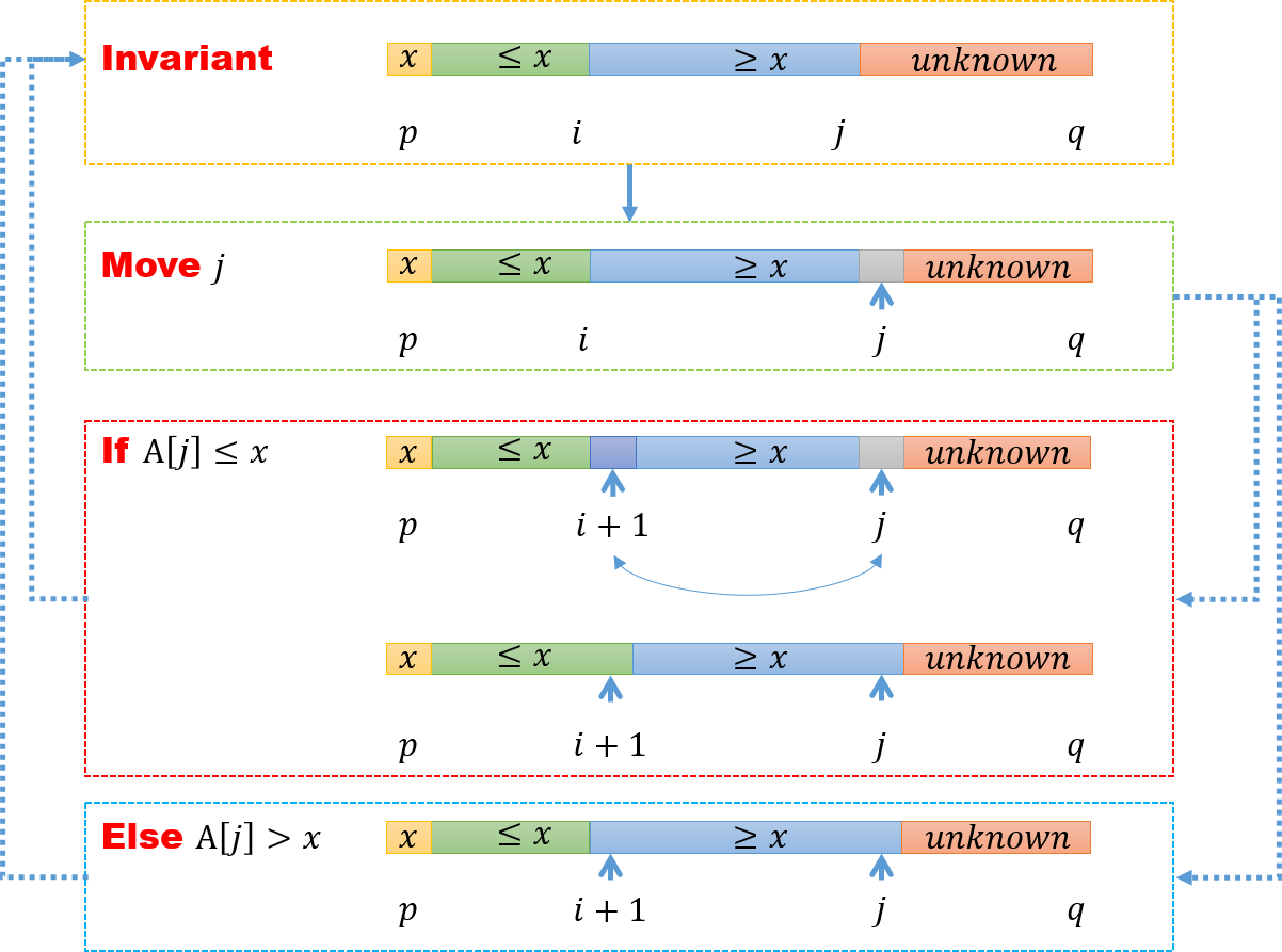
Actually, we hold our array with 4 area (but some of them maybe empty), which is also our “invariant”. The first area is the first element ${ x }$. And, all the elements of the second area is less than or equal to ${ x }$. The third area include some elements which are greater than ${ x }$. The last area is called “unknown area”, the elements in which are undecided.

In each loop, when we move to next element, we first compare it to ${ x }$, if it’s greater than ${ x }$, then we continue move forward. If not, we exchange it with the first element in third area (all the elements in it is greater than ${ x }$). So, in the second situation, the second area is entended by one element, and the hole third area move forward by one element.

When the index ${ j }$ move to ${ q }$. Then the unknown area is a empty set. At that time, we have three area: ${ x }$, second area (${ \leq x }$) and third area (${ \geq x }$).

In the end, we exchange the first element ${ A[p], x }$ with the last element of second area. We will find, all the elements which is less than ${ x }$ list in the left of ${ x }$, and the all the elements greater than ${ x }$ are positioned in the right of the ${ x }$.

It’s easy to check the runting time of “Partitioning” is ${ \Theta(n) }$.

Runing time Analysis

Then we can write down the pseudocode of Qiucksort

1
2
3
4
5
6
7
8
Quicksort(A,p,q): // treat A[p···q]
    if p < q
        r = Partition(A,p,q)
        Quicksort(A,p,r-1)
        Quicksort(A,r,q)

//Initial Call
Quicksort(A,1,n)

Worst-case analysis

Here, to analyze the runing time of Quicksort, we assume all the elements is distinct (not redundant). Let’s ${ T(n) }$ be the worst-case runing time. So, if the input array is sorted or reverse sorted, the partitioning is the worst case, becasue one side of the partition has no elements. Here we can right the recursion of Quicksort (the runting time of empty side is ${ T(0) }$, and the another side is ${ T(n-1) }$, the partition time is ${ \theta(n) }$)

Best case Analysis

In general, we don’t do best-case analyses, but here we do it for intuition only. If we are in the lucky case, Partition splits the array ${ n/2 : n/2 }$. In this case, the recursion is

1:9 Split?

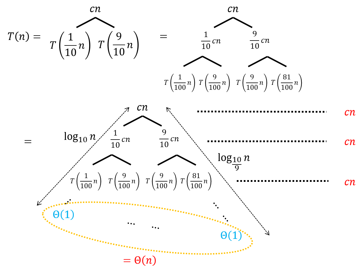
But, how about Split is always ${ 1/10 : 9/10 }$? We are in lucky or unlucky case? Let’s draw a recursion tree for this (denote ${ \Theta(n) }$ as ${ cn }$)

Form the recursion tree, we can observe the range of the running time is

And, we surprisingly find, ${ T(n) =\Theta( n \lg n )}$. We are in the lucky case!!

Alternative partition

Suppose, we are alternatively in lucky and unlucky case. What’s happen? We can first wirte down the recurrences of Lucky (${ L(n) }$) and Unlucky case (${ U(n) }$)

Then, we can use the recurrence of ${ U(n/2) }$ plug in the ${ L(n) }$, that gives us

But anyway, even we are alternatively in lucky partition, we still have a ${ \Theta(n \lg n) }$ running time. Now, we proposed another question, how can we avoid unlucky case?

We can randonmly arrange the elements OR randomly choose the pivot!

Randonmized Quicksort

Here we choose the last way to do, becasue it’s easy to analyze the running time.

• Pivot on random element (we swap the first element with some other element in the array before partition)

• The running time is independent of the input ordering.

• No assumptions about the input distribution.

• No specific input can elicit the the worst-case behavior.

• Worst-case determined only by random number generator.

Analysis of runing time

Let ${ T(n) }$ be the random variable for the runing time, assuming the random numbers are independent.

For a particular partition ${ k=0,1,\cdots, n-1 }$, we have the corresponding indicator random variable ${ x_k }$

So the expectation of ${ x_k }$ is

And the recurrence of ${ T(n) }$ is

Or we can use a little trick to treat the ${ T(n) }$ as following

Then, we gonna talk about the Expectation of ${ T(n) }$

Here we need to notice that ${ \sum_{k=0}^{n-1} E\left[T(k)\right]=\sum_{k=0}^{n-1} E\left[T(n-k-1)\right] }$, they are just in different order. So, we can get

For technical convenience, we want to absorb the ${ k=0,1 }$ terms in to ${ \Theta(n) }$. (Why we do that? We can get it in the following step). Actually, ${ E\left[T(1)\right], E\left[T(2)\right] }$ are just constants, so it can be absorb into ${ \Theta(n) }$, that is

So, we have done all the simplification for recurrence, now we solve it! We are going to prove ${ E\left[T(n)\right] \leq an\lg n }$ for some contant ${ a>0 }$. How can we do it?? Substitution Method!!

Choose ${ a }$ big enough so that ${ a n \lg n \geq E\left[T(n)\right]}$ for some small ${ n }$. (That’s the reason why we absorb ${ k=1,0 }$ items, because they will never make the cases work)

We will use the fact that

By assumption, the expectation of running time satisfies

By use the fact above, we get

Here, if ${ a }$ is big enough such that ${ \frac{an}{4} > \Theta(n) }$, we can get ${ E\left[T(n)\right] \leq a n \lg n}$.