Heapsort
In this exercise part, we gonna introduce Heapsort. Heapsort’s running time is ${ O (n\lg n) }$. Just like Quicksort, heapsort sorts array in place.
Heapsort also introduce aother useful algorithm design techinque: a kind of data structure called “heap”. Here the “heap” can be used in Heapsort and Priority queue. Let’s move forward to its content!
Heap
The (binary) heap data structure is an array object that we can view as a nearly complete binary tree. An array ${ A }$ that represents a heap is an object with two attributes: ${ A.length }$, which (as usual) gives the number of elements in the array, and ${ A.heap-size }$, which represents how many elements in the heap are stored within array ${ A }$. That is ${ 0 \leq A.heap-size \leq A.length}$
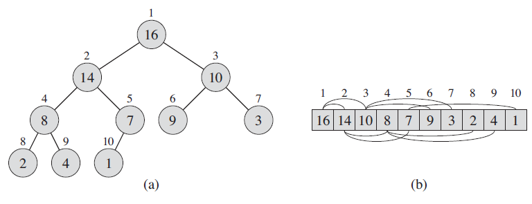
An example of Heap1
For each note ${ i }$, we can easily compute the indices of its parent, left child and right child:
1
2
3
4
5
6
PARENT (i)
    return [i/2]
LEFT (i)
    return 2i
RIGHT (i)
    return 2i+1
It's easy to check the anwser!
--- Suppose note ${ i }$ is the ${ x^{th} }$ note in the ${ k^{th} }$ level. So, ${ i = \sum_{j=1}^{k-1} 2^{j-1} +x = 2^{k-1} - 1 +x }$. For the left child of note ${ i }$, the number of notes from ${ 1^{st} }$ to ${ k^{th} }$ level is ${ 2^{k} - 1 }$, and the remaining notes before left child in ${ (k+1)^{th} }$ level is ${ [2(x-1) + 1]^{th} }$ note. So the order of left child is ${ 2^{k} - 1 + 2x -2 + 1 = 2^{k} + 2x -2 = 2i}$. So, it's easy to check the indices of right child and parent. ---There are two kinds of binary heaps: max-heaps and min-heaps. In a max-heap, the max-heap property is that for every node ${ i }$, other than the root,
That means the largest value is stored at the root (Note: we use max-heap in Heapsort algorithm). A min-heap is organized in the opposite way: the min-heap property is that for every node ${ i }$ other than the root,
The smallest element in a min-heap is at the root. And, it’s easy to check the height of the tree is ${ \Theta(\lg n) }$.
In the following, we gonna talk about how Heapsort works. We have several proceduces
-
MAX-HEAPIFY proceduce, which runs in ${ O(\lg n) }$ time, is the key to maintaning the max-heap property.
-
BUILD_MAX_HEAP procedure, which runs in linear time, procedures a max-heap from an unordered input array.
-
The HEAPSORT procedure, which runs in ${ \Theta(n \lg n) }$ time, sorts an array in place.
Maintaining the heap property
Assume that the binary trees rooted at ${ \text{LEFT}(i) }$ and ${ \text{RIGHT}(i) }$ are max-heaps, but that ${ A[i] }$ might be smaller than its children. So we can call Max-property here to maintain the heap property, the pseudocode is shown below
1
2
3
4
5
6
7
8
9
10
11
12
MAX-HEAPIFY(A,i)
    l = LEFT(i)
    r = RIGHT(i)
    if l <= A.heap-size and A[l] > A[i]
        largest  = l // "largest" stores the index of largest element
    else
        largest = i
    if r <= A.heap-size and A[r] > A[largest]
        largest = r
    if largest != i
        exchange A[i] with A[largest]
        MAX-HEAPIFY(A, largest)
The idea of MAX-HEAPIFY is clear, we just compare the value of ${ A[i], A[r], A[l] }$, if ${ A[i] }$ not the largest one, we exchange it to the largest one of its children. The exchange may cause that the binary heap of ${ A[largest] }$ violates the heap property, so we need to call MAX-HEAPIFY recursively on that subtree.
Now, we analyze the running time of MAX-HEAPIFY for a tree with ${ n }$ notes, the cost of this procedure is from the exchange time ${ \Theta(1) }$ and the time to recursively run MAX-HEAPIFY on a subtree.
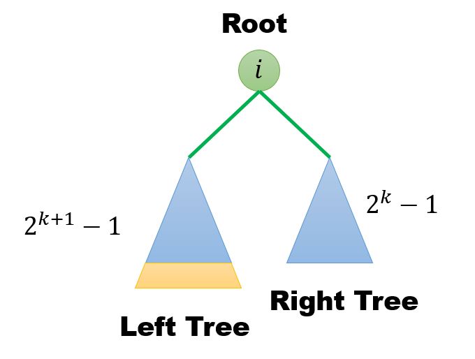
The worst case of runing MAX-HEAPIFY on subtree happens when the bottom level of the tree is exactly half full. The children's subtrees have size at most ${ 2n/3 }$.
--- For the binary tree at root ${ i }$, the worst case is that the left subtree takes a biggest part of the whole tree, which means the left subtree contains one more level than right subtree. We can suppose the height of right subtree is ${ k }$, so the number of left subtree and right subtree are ${ 2^{k+1}-1 }$ and ${ 2^k -1 }$, so the ratio of left subtree over whole tree isTherefore, the recurrence of ${ T(n) }$ is
Accoding to Master Theorem case 2, ${ n^{\log_{3/2} 1 } = 1}$, ${ f(n) = \Theta(1 (\lg n)^{0}) }$. So, ${ T(n) = O(\lg n) }$
Building a heap
We can use the procedure MAX-HEAPIFY in a bottom-up manner to convert an array ${ A[1…n] }$, where ${ n = A.length }$, into a max-heap. For all the leaves, they are already a max-heap with just one element. And, we can call MAX-HEAPIFY to rearrange the PARENT of these leaves. From bottom to the root, we can build a max-heap. Here we put up the pseudo code of BUILD-MAX-HEAP
1
2
3
4
BUILD-MAX_HEAP(A)
    A.heap-size = A.length
    for i = [A.length/2] downto 1
        MAX-HEAPIFY(A,i)
We can easily check the indices of leaves are ${ \lfloor n/2 \rfloor + 1, \lfloor n/2 \rfloor + 2, \cdots, n }$. So, the loop begins from ${ \lfloor A.length/2 \rfloor }$
--- For node ${ n }$, we know it's the last leaf in the tree, so its PARENT is the last note which has a child / children. So, the first leaves number is ${ \text{PARENT}(n) + 1 = \lfloor n/2 \rfloor + 1}$ ---For BUILD-MAX-HEAPIFY procedure, we can calculate the total cost of its runing time. We already know the runing time of MAX-HEAPIFY is ${ O(\lg n) }$, if we denote the height of tree as ${ h }$, the runing time is ${ O(h) }$.
Because we call MAX-HEAPIFY from bottom to root, in each level, the number of notes whose height are ${ h }$ is ${ \lceil \frac{n}{2^{h+1}} \rceil}$.
--- Because, the notes whose height is ${ h }$, means they lay in the ${ \lfloor \lg n \rfloor ^{th} - h}$ or ${ (\lfloor \lg n \rfloor - 1 - h )^{th} }$. So, there are at most ${ \lceil2 ^ {\lfloor \lg n \rfloor ^{th} - h - 1} \rceil = \lceil \frac{n}{2^{h+1}} \rceil}$ notes whose height is ${ h }$ (Note, the ${ k^{th} }$ level have ${ 2^{k-1} }$ notes). ---Therefore, we can get the running time
Thus, through our analysis, the runing time of BUILD-MAX-HEAP is linear.
Heapsort Algorithm
We use BUILD-MAX-HEAP to make ${ A[1…n] }$ into a max-heap. And, we can exract ${ A[1] }$ which is already the largest element. We exchange ${ A[1] }$ and ${ A[n] }$. Then, we consider the array ${ A[1…n-1] }$, in this time, the root is ${ A[1] }$, which may not satisfy max-heap property, but the two subtree still statisfy it, and we can maintain it by MAX-HEAPIFY. Keep doing it, until the heap-size downto 2. Here is the pseudocode
1
2
3
4
5
HEAPSORT(A)
    for i = A.length downto 2
        exchange A[1] with A[i]
        A.heap-size = A.heap-size - 1
        MAX-HEAPIFY(A,1)
It’s easy to check the runing time is ${ T(n) = O(n) + n O(\lg n) = O(n \lg n) }$.
Priority queues
A priority queue is a data structure for maintaining a set ${ S }$ of elements, each with an associated value called a key. A max-priority queue supports the following operations:
${ \text{INSERT}(S,x) }$ inserts the element ${ x }$ into the set ${ S, }$ which is equivalent to the operation ${ S = S \cup {x}. }$
${ \text{MAXIMUM}(S) }$ returns the element of ${ S }$ with the largest key.
${ \text{EXTRACT-MAX}(S) }$ removes and returns the element of ${ S }$ with the largest key.
${ \text{INCREASE-KEY}(S,x,k) }$ increases the value of element ${ x }$’s key to the new value k, which is assumed to be at least as large ${ x }$’s current key value.
Each object will correspond to an element in priority queue. Therefore, we often need to store a handle to record the mapping. Here, we don’t care about it, in fact when we move the an element in array, we need update the index for the corresponding object. Now, let’s introduce the procedures in detail.
- ${ \text{HEAP-MAXIMUM} }$ it can implement the ${ \text{MAXIMUM} }$ operation in ${ \Theta(1) }$ time. Here’s the pseudocode
1
2
HEAP-MAXIMUN(A)
    return A[1]
- ${ \text{HEAP-EXTRACT-MAX} }$ Procedure implement the ${ \text{EXTRACT-MAX} }$ operation, it’s similar to the ${ \text{HEAPSORT} }$ procedure.
1
2
3
4
5
6
7
8
HEAP-EXTRACT-MAX(A)
    if A.heap-size < 1
        error "heap underflow"
max = A[1]
A[1] = A[A.heap-size] // move the last heap element to the first
A.heap-size = A.heap-size - 1
MAX-HEAPIFY(A,1) // maintain the max-heap properties
return max
So, the main runing time takes on ${ \text{MAX-HEAPIFY} }$ procedure, therefore the cost ${ T(n) = O(\lg n) }$
The procedure ${ \text{HEAP-INCREASE-KEY} }$ implements the ${ \text{INCREASE-KEY} }$ operation. Becasue the key of ${ A[i] }$ increases, the max-heap properties may be violated. The idea of ${ \text{HEAP-INCREASE-KEY} }$ is similar with ${ \text{MAX-HEAPIFY} }$. In each time, we compare the value of current elements to its PARENT node, and adjust it if necessary. Then we put up the procedure
1
2
3
4
5
6
7
HEAP-INCREASE-KEY(A,i,key)
    if key < A[i]
        error "new key is smaller than current key"
    A[i] = key
    while i > 1 and A[PARENT(i)] < A[i]
        exchange A[i] with A[PARENT(i)]
        i = PARENT(i) // keep changing until satisfy heap properties
It’s easy to check the runing time is ${ O(\lg n) }$, due to the length between node ${ i }$ and finnal position is less than height of heap ${ \lg n }$
The procedure ${ \text{MAX-HEAP-INSERT} }$ implements the ${ \text{INSERT} }$ operation. The idea of inserting an element and keeping the max-heap properties is first adding a leaf with ${ -\infty }$ as its key. And, call ${ \text{HEAP-INCREASE-KEY} }$ procedure.
1
2
3
4
MAX-HEAP-INSERT(A,key)
    A.heap-size = A.heap-size + 1
    A[A.heap-size] = -∞
    HEAP-INCREASE-KEY(A,A.heap-size,key)
The main cost in this procedure is at ${ \text{MAX-HEAP-INSERT} }$, so the runing time is ${ O(\lg n) }$. Therefore, all the operation can be finished in ${ O(\lg n) }$ time.
Hat-check problem
Use indicator random variables to solve the following problem, which is known as the hat-check problem. Each of ${ n }$ customers gives a hat to a hat-check person at a restaurant. The hat-check person gives the hats back to the customers in a random order. What is the expected number of customers who get back their hats?
Let ${ X_i }$ be the indicator random variable that indicates whether the customer ${ i }$ gets his hat back
So, the number of customers who get their hats back is ${ \sum_{i=1}^n X_i}$. Therefore the expected number is
Is this almost sorted?
In this problem, we wants to know whether 90% of the elements are sorted: is it possible to remove 10% of the elements and have the resulting list be sorted?
In this problem, we will find an algorithm that takes as input a list ${ A }$ containing ${ n }$ distinct elements, and acts as follows:
- If the list ${ A }$ is sorted, the algorithm always returns true.
- If the list ${ A }$ is not 90% sorted, the algorithm returns false with probability at least ${ 2/3 }$.
Problem (a)
First considers the following algorithm:
Repeat k times:

1. Choose an element ${ i }$ and uniformly at random from the open interval ${ (1,n) }$.(That is, ${ 1 < i < n  }$)
2. Compare element ${ A[i-1] }$ and ${ A[i] }$. Output <b>false</b> and halt if they are not sorted correctly.
3. Compare element ${ A[i] }$ and ${ A[i+1] }$. Output <b>false</b> and halt if they are not sorted correctly.

Output <b>true</b>
Show that for this algorithm to correctly discover whether the list is almost sorted with probability at least ${ 2/3 }$ requires ${ k = \Omega(n) }$. Hint: Find a sequence that is not almost sorted, but with only a small number of elements that will cause the algorithm to return false.
Answer:
The big picture of the idea to prove is find a List that be determind correctly with probability at least 2/3 requires ${ k = \Omega(n) }$. Here we will construct a list that is not 90% sorted, but only a small number of elements will cause Snape’s Algorithm return false, that means it’s hard to determine this list is not 90% sorted. To get the probability, we have to increase ${ k }$.
Ok, here we consider the following example
Lemma 1 ${ A }$ is not 90% sorted
Proof. Assume ${ A }$ is 90% sorted. That means there must be some 90% elements that are correctly sorted. It’s easy to check, the first half and second half of the list are already sorted. And, these 90% elements have to contain the elements in first half and elements in second half. But, any elements in first half are greater than any elements in second half, which contradicts with 90% elements are sorted. By contradiction, ${ A }$ is not 90% sorted.
Lemma 2 For list ${ A }$, Snape’s algorithm returns false with probability at least 2/3 requires ${ k = \Omega(n) }$
In each interation, this algorithm returns false only in two cases, ${ i = \lfloor n/2 \rfloor }$ or ${ i = \lfloor n/2 \rfloor + 1 }$. Define indicator random variables as follows:
Therefore, ${ Pr{X_{ell} = 1} = 2/n }$ and ${ Pr{X_{ell} = 0} = 1- 2/n }$. To let the probability of returing false at least 2/3, we need the probability of returning true less than 1/3. That is
Solving ${ k }$ as follow,
We use following fact
Therefore,
Therefore, ${ k= \Omega(n) }$.
Problem (b)
Imagine you are given a bag of ${ n }$ balls. You are told that at least 10% of the balls are blue, and no more than 90% of the balls are red. Asymptotically (for large ${ n }$) how many balls do you have to draw from the bag to see a blue ball with probability at least ${ 2/3 }$? (You can assume that the balls are drawn with replacement.)
Anwser: Denote the ratio of blue balls in the bag as ${ r_b }$, which is greater than 10%. And the ratio of red balls is ${ 1 - r_b }$, which is less than 90%.
So, our task is to prove how many times ${ k }$ we need to let the probability of picking up a blue ball at least ${ 2/3 }$. In other word, we need the probability of picking up a red ball in each time less than ${ 1/3 }$.
Define indicator random variables as follows:
So, ${ Pr \left( X_i = 0 \right) = 1 - r_b < 0.9 }$. Therefore, we need to calculate ${ k }$ to satisfy ${ \prod_{i=1}^k Pr \left( X_i = 0 \right) < 1/3 }$, that is
Therefore, ${ k > \frac{\ln (1/3)}{\ln 0.9} }$, the probability of drawing at least one blue ball is at least 2/3.
Problem (c)
Consider performing a “binary search” on an unsorted list:
1
2
3
4
5
6
7
BINARY-SEARCH(A, key, left,right) \\ Search for key in A[left . .right].
    if left = right
        then return left
    else mid ← int[(left + right)/2] + 1
        if key < A[mid]
            then return BINARY-SEARCH(A, key, left, mid − 1)
        else return BINARY-SEARCH(A, key, mid,right)
Assume that a binary search for ${ key_1 }$ in ${ A }$ (even though ${ A }$ is not sorted) returns slot ${ i }$. Similarly, a binary search for ${ key_2 }$ in ${ A }$ returns slot ${ j }$. Explain why the following fact is true: if ${ i < j }$, then ${ key_1 < key_2 }$. Draw a picture. Hint: First think about why this is obviously true if list ${ A }$ is sorted.
Anwser: For ${ key_1 }$, denotes all the elements that are compared against ${ key_1 }$ in line 4 in order as ${ x_1, x_2, \cdots, x_p }$. Similarly, denotes the elements compared against ${ key_2 }$ as ${ y_1, y_2, \cdots, y_q }$. For first comparison, ${ x_1 = y_1 = A[\lceil n/2 \rceil] }$. So, we have two kinds of cases.
Case 1. ${ A[\lceil n/2 \rceil] }$ is between ${ key_1, key_2 }$. Obviously, ${ key_1 < x_1 = y_1 = A[\lceil n/2 \rceil] < key_2 }$. If not, assume ${ key_2 < A[\lceil n/2 \rceil] < key_1 }$, then ${ key_2 }$ will search in the left of array ${ A }$ and ${ key_2 }$ in right, which contradicts to ${ i < j }$. Because ${ key_1 < A[\lceil n/2 \rceil] < key_2 }$, the slot ${ i }$ are located in left array and slot ${ j }$ lies on right array. Hence, we get ${ i < j }$.
Case 2. ${ key_1, key_2 }$ are both larger or smaller than ${ A[\lceil n/2 \rceil] }$. Therefore, we can move to next comparison, and ${ x_2 = y_2}$. We still have two cases just like Case 1 and Case 2.
Let ${ \ell }$ as the smallest number such that ${ x_\ell \neq y_\ell }$, we can get
Hence, we get the conclusion ${ i < j }$.
Problem (d)
Professor Snape proposes a randomized algorithm to determine whether a list is 90% sorted. The algorithm uses the function ${ \text{RANDOM}(1,n) }$ to choose an integer independently and uniformly at random in the closed interval ${ [1,n] }$. The algorithm is presented below.
1
2
3
4
5
6
7
IS-ALMOST-SORTED(A,n,k) \\ Determine if A[1...n] is almost sorted.
    for r ← 1 to k
        do i ← RANDOM(1,n) \\ Pick iuniformly and independently.
            j ← BINARY-SEARCH(A,A[i],1,n)
            if i != j
                then return false
    return true
Show that the algorithm is correct if ${ k }$ is a sufficiently large constant. That is, with ${ k }$ chosen appropriately, the algorithm always outputs true if a list is correctly sorted and outputs false with probability at least ${ 2/3 }$ if the list is not 90% sorted.
Anwser:
Problem 1: If the list ${ A }$ is sorted, the algorithm always returns true.
Proof. Due to the correctness of Binary Search in a sorted array. And input list ${ A }$ contains ${ n }$ distinct elements. Therefore, ${ j }$ will always equal to ${ i }$, The algorithm will return true.
Problem 2: If the list ${ A }$ is not 90% sorted, the algorithm returns false with probability at least ${ 2/3 }$.
For randomly extracted element ${ i }$, we label the elements as “good” or “bad” as follow:
Lemma 3: If the list ${ A }$ is not 90% sorted, then at least 10% of the elements are bad.
Proof. Assume, by contradiction, that fewer than 10% of the elements are bad. Then, at least 90% elements are good. Remove all the bad elements from the array, which is less than 10%. Consider any two elements in remaining array ${ key_1 }$ and ${ key_2 }$, where ${ key_1 }$’s index is ${ i }$, ${ key_2 }$’s index is ${ j }$. Because they are “good”, so we can guarantee the Binary Search result will return slot ${ i,j }$ for ${ key_1,key_2 }$. From Problem (c), we know if ${ i<j \Rightarrow key_1 < key_2}$, if ${ i>j \Rightarrow key_1 > key_2}$. That means ${ key_1, key_2 }$ are sorted. Because, any two elements in array are sorted, so the remaining array are sorted. Therefore, original list is a 90% sorted array, which contradicts to conditon.
Lemma 4: If the list ${ A }$ is not 90% sorted, the algorithm returns false with probability at least ${ 2/3 }$.
Proof. From lemma 4, we know the “bad” elements are greater than 10%. From Problem (b), we know if we choose ${ k > \ln (1/3) / \ln (0.9) }$, then we will find a bad element with probability at least 2/3.
Problem (e)
Imagine instead that Professor Snape would like to determine whether a list is ${ 1 − \epsilon }$ sorted for some ${ 0 < \epsilon <1 }$. (In the previous parts ${ \epsilon= 0.10 }$.) For large n, determine the appropriate value of k, asymptotically, and show that the algorithm is correct. What is the overall running time?
Proof. Similarly, we know if a list is not ${ 1 − \epsilon }$ sorted, we will have at least ${ \epsilon n }$ “bad” elements. We still denote the retio of bad elements as ${ r_b > \epsilon }$, so the we need choose ${ k }$ to satisfy
${ \Leftarrow (1-\epsilon)^k \leq \frac{1}{3}}$ ${ \Leftarrow (1-\epsilon)^k \leq \frac{1}{e^2}}$
We can solve ${ k }$
If we choose ${ k = 2/\epsilon }$, we will find ${ k }$ satisfis the above equation.
Here we use the fact ${ \ln(1+x) \leq x , x > -1}$
And the runing time of Binary Search is ${ O(\lg n) }$, so the runing time of Snape’s Algorithm is ${ O(\lg n / \epsilon) }$.
-
Cormen, T. H., Leiserson, C. E., Rivest, R. L., & Stein, C. (2022). Introduction to algorithms. MIT press. ↩