This blog is talking about how to solve linear optimization problems involving two decision variables graphically.

LO problems involving 2 variables

Consider a linear function ${ f:\mathbb{R}^2 \rightarrow \mathbb{R} }$

$$ f(\bar{x}) = \bar{c}^T \bar{x} $$

Let’s look at the level sets of the function ${ f }$.

$$ f^{-1}(0) = \{\bar{x}| 0=f(\bar{x} \} = \{\bar{x}| 0=\bar{c}^T \bar{x} \} $$

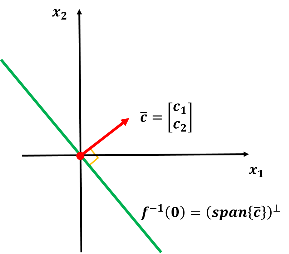
In fact, all the points that satisfy ${ f(\bar{x}) = 0 }$ form a line that is perpendicular to ${\bar{c} }$ (here ${ \bar{c} \neq \bar{0}}$). So, we can have

$$ f^{-1}(0) = (\text{span}\{\bar{c}\})^{\perp} $$

Observation: Two vectors ${ \bar{p},\bar{q} \in \mathbb{R}^2 }$ are in the same level set of the linear function ${ f }$ iff

$$ f(p) = f(q) \\ p - q \perp \bar{c} $$

Thus the level set of function ${ f = c^T x }$ are the linear orthogonal to ${ span{\bar{c}} }$

What is the value set of linear function ${ f=c^Tx }$ associate with value ${ K }$

$$ x \in f^-1(K) \Leftrightarrow f(x) = K $$ $$ \Vert c \Vert \Vert x \Vert \cos \theta = K $$ $$ \Vert x \Vert \cos \theta = \frac{K}{\Vert c \Vert} $$

Hence ${ f^-1(K) }$ is the linear orthogonal to ${ span{c} }$ located at signed distance ${ \frac{K}{\Vert c \Vert} }$ from the origin (${ \bar{0} }$) in the directio of ${ \bar{c} }$

Draw the solution of the linear inequality ${ 2x_1+ x_2 \geq 6 }$

It’s the union of all the level sets of the linear function ${ (x_1,x_2) \mapsto 2x_1 + x_2 }$ corrsponding to all the values ${ 6 }$ and higher

• STEP 1: Draw boundry line ${ 2x_1+ x_2 = 6 }$.

• STEP 2: Draw normal vector ${ \left[\matrix{2 & 1}\right]^\top }$. Along the direction of normal vector, the value of ${2x_1 + x_2 }$ increases.

• STEP 3: Draw the half plane.