The spatial transcriptome is a novel and cutting-edge field and can identify single-celler transcriptome and corresponding locations. This paper reviews the current statistical and machine-learning methods in Spatial transcriptome. And it’s also my first paper read in this field. First, let us introduce the wet-lab technologies in this area to show what spatial transcriptome is.

Intro to Spatial Transcriptome Technologies

Why do we need ST? Single-cell RNA-seq can provide a perspective on the gene expression level at a cell level. But, when we prepared the sequencing for a single cell, we lost all the information of its location in vivo. The cell position is critical to identify the cell type, state, and function for us. Moreover, many cell communications are based on surface-bound protein receptor-ligand pairs, meaning many signals are passed via neighboring cells or in the same tissue. However, we should give scRNA-seq an objective evaluation that this technology has permitted unbiased(i.e., characterizing the expression of every gene in the genome), genome-scale assessments of cellular identity, heterogeneity, and dynamic change for thousands to hundreds of thousands of cells ¹.

Broadly, there are two ways to complete the goal of detecting transcriptome while preserving location information. Actually, the development of Spatial Transcriptome technologies has lasted for decades, and there are many technologies to pursue this aim. If you are interested, move to this review or this blog to learn more details about the history of ST.

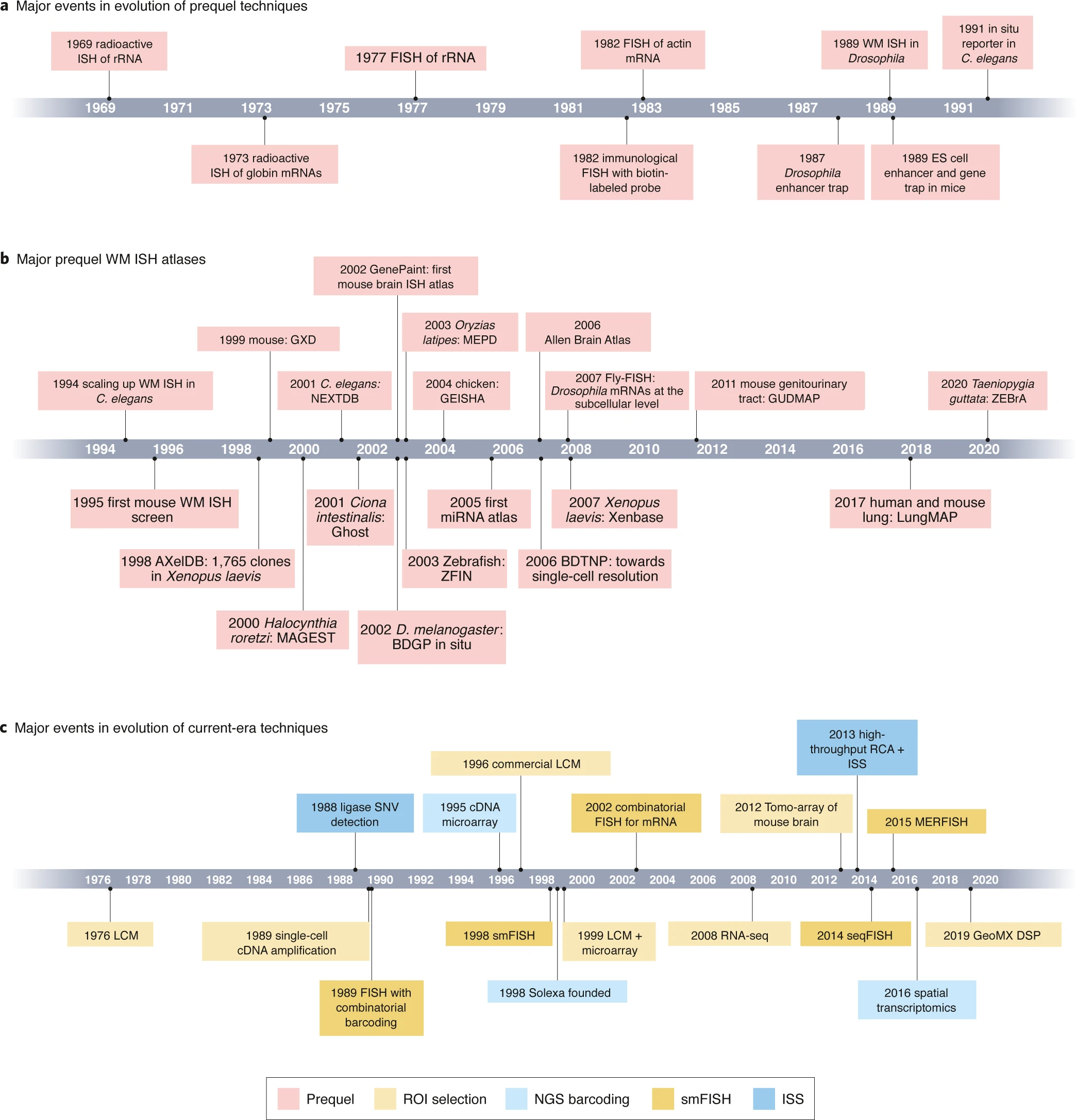
Fig.1 Timeline of Spatial Transcriptome Technologies.²

The first class of methods is image-based, including in situ hybridization (ISH) and in situ sequencing (ISS). ISH methods use gene-specific fluorophore-labeled probes to detect the number of target mRNAs that we have known their sequence, which means we can only identify a few already-known mRNAs in tissue. In terms of ISS, we use fluorophore-labeled bases to amplify transcripts in situ and obtain their sequences. This technology seems perfect for obtaining sequences and positions at the same time. But actually, the read in FISSEQ (a kind of technology of ISS) is around 5-30nt, and only 200 mRNA reads were captured per cell. Compared to it, 40,000 mRNA reads were detected in scRNA-seq.

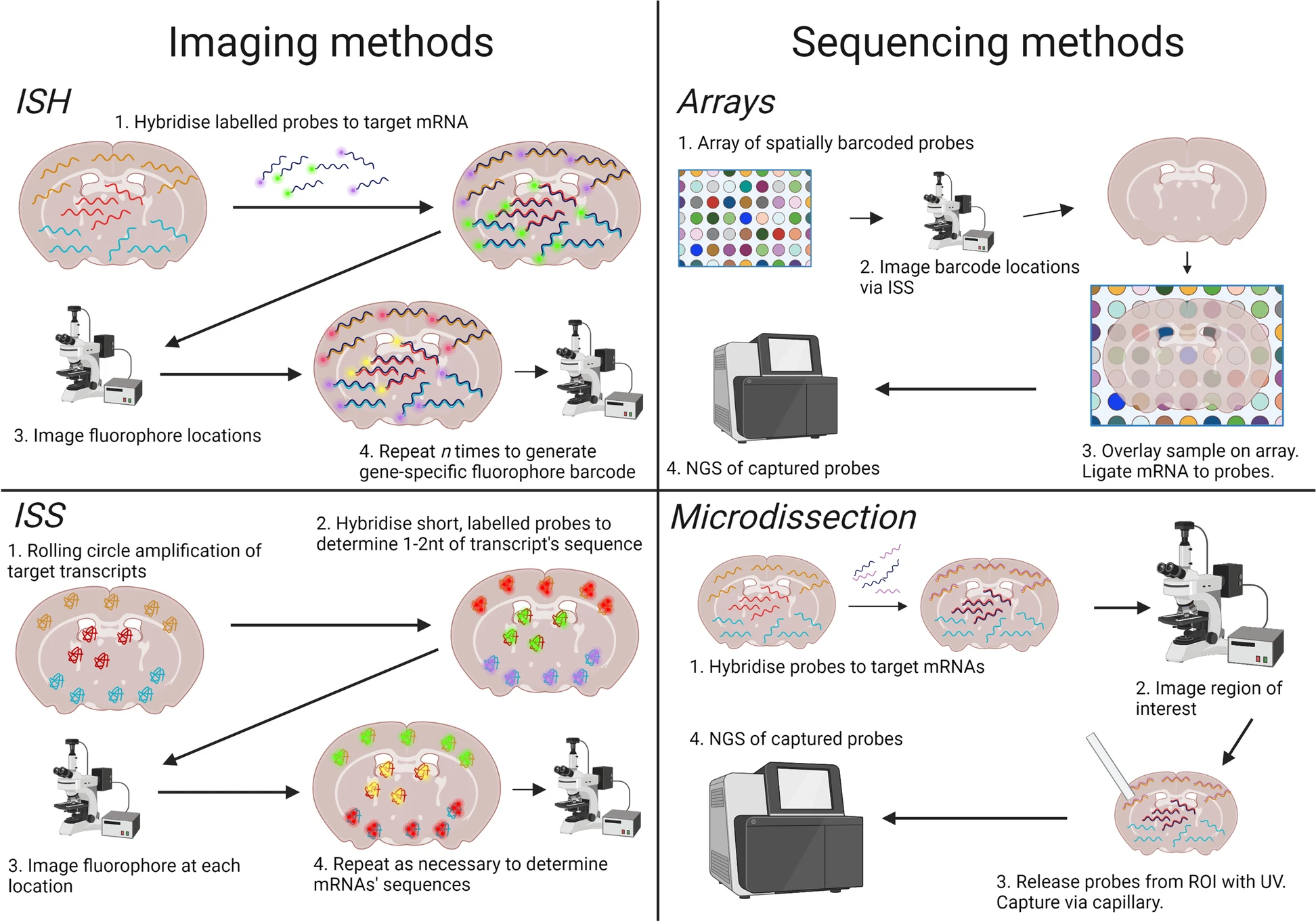
Fig.2 Classes of Spatial Transcriptome Technologies.¹

In fact, the most popular and current Spatial Transcriptome Technologies belong to the sequence-based class. The early technology was Laser Capture Microdissection (LCM). Through the laser (like IR or UV), we can section the tissue into small pieces and detect the RNA-seq for each piece. It still has some disadvantages, such as limited resolution and laborious process. Alright, let’s focus on the most advanced and common technology in recent years–the array-based methods.

Tissue was mounted over an array, such that released mRNA was captured locally by spatially-barcoded probes, converted to cDNA, and then sequenced¹. Actually, in human body, the diameter of cell is around 5-200 ${ \mu m }$ (typically 5-10 ${ \mu m}$). A disadvantage of these methods is that capture areas do not follow the complex contours of cellular morphology. Hence, cells often straddle multiple capture areas, contributing mRNA to more than one pixel. Even when capture areas are smaller than a single cell (as in HDST), they still lack single-cell resolution, since they capture mRNA merely from a single-cell-sized area. Besides, their spatial resolution and mRNA recovery rates are lower than ISH and ISS-methods. Finally, by relying on a fixed array, transcripts from different cells can be captured at the same spot, meaning that sophisticated analyses are needed to determine what cell types were present at each spot. The process of identifying and quantifying the relative contribution from each cell type in a capture spot is known as deconvolution¹.

In summary, spatial transcriptomics retains spatial information, but majority of the data is neither transcriptome-wide (e.g., Slide-seqV2 recovers ~ 30–50% as much transcriptomic information per capture bead as droplet-based single-cell transcriptomics from 10X Genomics¹) in breadth nor at cellular resolution in depth. Indeed, by leveraging both expression profiles from scRNA-seq data and spatial patterns from spatial transcriptomics data, we can transfer knowledge between the two types of data, which benefits the analysis of both data types. It has been shown that the integration of scRNA-seq and spatial transcriptomics data could improve model performance in different research areas³.

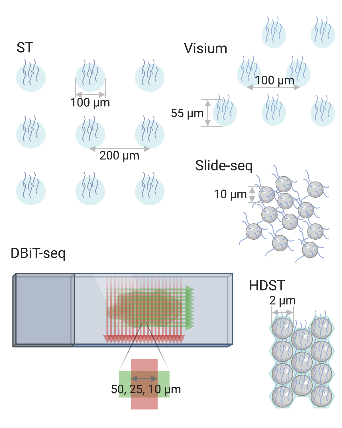
Fig.3 Array-based Technologies.⁴

Overview of Spatial Transcriptome Workflow.

In this part, I will follow the sections in the paper, showing the computational task in the process of Spatial Transcriptome data analysis.

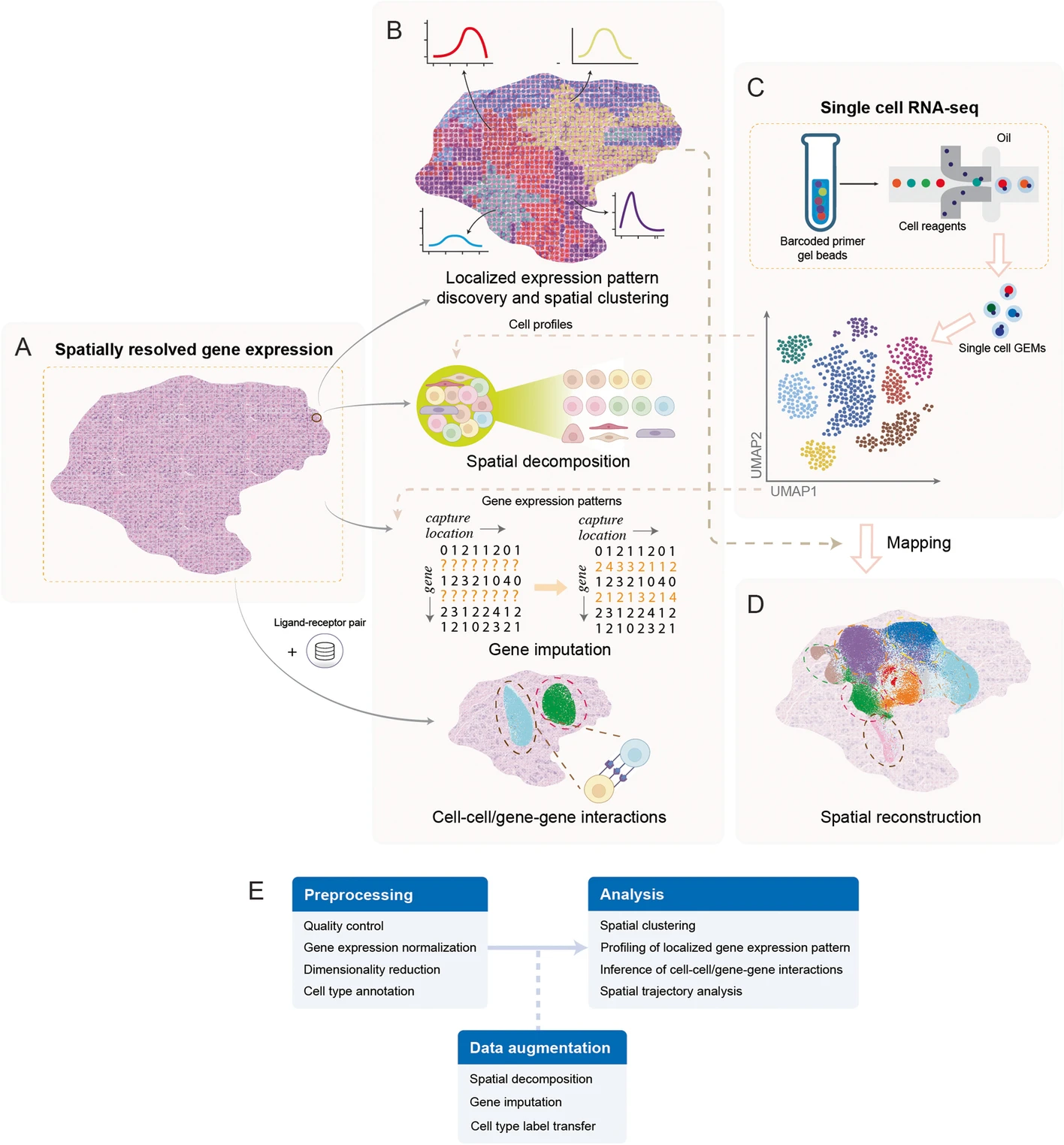
Fig.4 Sspatial transcriptomics data analysis workflow.³

Profiling of localized gene expression pattern

The spatial expression pattern (also called Spatially Variable Genes, SVGs) of a given gene can be detected using statistical or machine learning methods. For statistical methods, they identify whether the gene expression corresponds to their location. Specifically, they test whether the gene expression is independent of their distance. We take SPARK-X⁵ as an example. SPARK-X first calculates the covariance matrixes for a given gene and Spatial coordinates. We use n to denote the number of locations, E as gene expression covariance, and S as the distance covariance matrix. We use ${ n }$ to denote the number of locations, ${ E }$ as gene expression covariance, and ${ \Sigma }$ as distance covariance matrix. Here we use following formula to test the independency between the given gene and cordianates.

$$ T = trace(E \Sigma) $$

We can treat it more intuitively. The matrix

$$ { E = \left[ \begin{matrix} g_1 \\ \vdots \\ g_n \end{matrix} \right]} \quad and \quad { \Sigma = \left[ \begin{matrix} s_1 & \cdots & s_n \end{matrix} \right]}. $$

So ${ T = \sum_i^n g_i s_i}$. Actually, ${ g_i,s_i }$ represent the Correlation between location ${ i }$ and other locations in expression level and distance, respectively. Therefore, the ${ g_i s_i }$ can represent the Correlation between the Correlation of expression level and distance. If the given gene is independent to Spatial cordianates, the ${ T }$ will be very small.

Another class is machine learning, and we take SpaGCN⁶ as an example. First, the SpaGCN constructs a graph for Spatial Transcriptome data, in which the node is locations/cells, and the edge weight is based on physical distance and histological information (which is an image and can be waived). Next, SpaGCN employs a layer of GCN to aggregate the information (gene expression vector) for each vertex via the graph. Then it utilizes an unsupervised clustering algorithm (Louvain algorithm) to identify Spatial domains. Finally, it can detect SVGs through DE analysis with target and other domain.

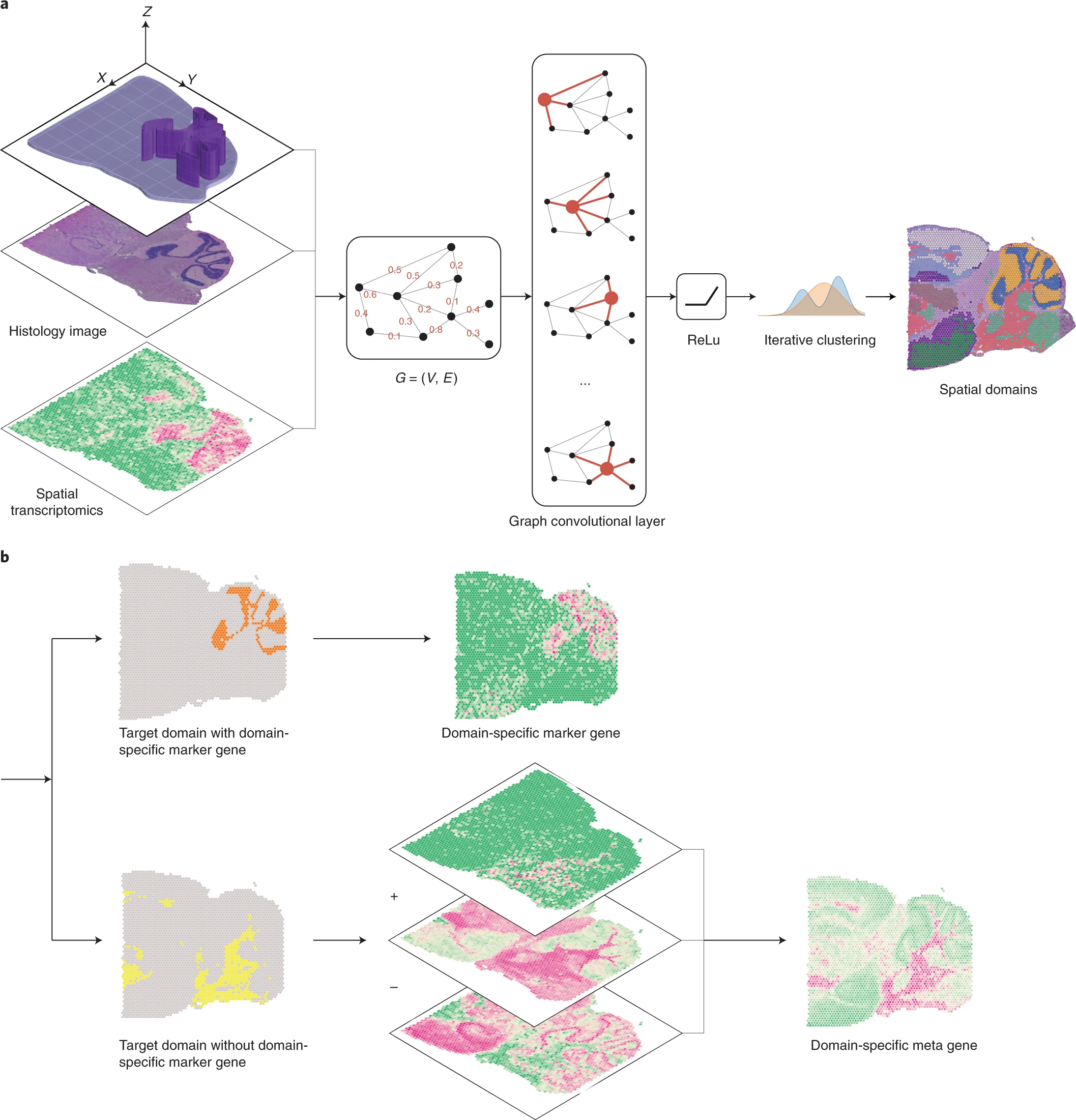
Fig.5 SpaGCN workflow.⁶

Spatial clustering

The profiling of localized gene expression patterns is closely related to delineating spatially connected regions or clusters in a tissue based on expression data. Indeed, spatial clustering is a critical step when performing exploratory analysis of spatial transcriptomics data, which may help reduce the data dimensionality and discover spatially variable genes³, like SpaGCN⁶. Most methods first process the Spatial Transcriptome data and then employ the clustering algorithm, like k-means or Louvain.

Spatial decomposition and gene imputation

Traditionally, cellular deconvolution commonly refers to estimating the proportions of different cell types in each sample based on its bulk RNA-seq data. Theoretically, methods designed for bulk RNA-seq data deconvolution could be adopted for spatial transcriptomics data. Here, we breifly introduce the method of DWLS⁷. We denote the bulk RNA-seq data as a vector ${ t = (t_1, \cdots ,t_n)^T}$. We can use scRNA-seq to get the gene expression situation of each type, which can build the matrix ${ S = (s_{ij})_{(n\times k)} }$, where ${ k }$ represents the number of types. So we want to solve the solution ${ x = (x_1, \cdots ,x_k)^T }$ satisfying the following equation

$$ Sx=t $$

But, ${ n \gg k }$, so the solution is non-determined, we can try to solve the following problem

$$ \mathop{\min}_{x} \Vert t-Sx \Vert $$

First, the estimation error for rare cell types is typically large since such a term has little impact on the total estimation error. Second, the contribution of a gene can be minimal if its mean expression level is low, even if it is highly differentially expressed between different cell types. To mitigate it, DWLS set weight in below formula

$$ \mathop{\min}_{x} \sum_{i=1}^n w_i(t_i-(Sx)_i)^2, w_i=\frac{1}{(Sx)_i} $$