From algorithms to tools – engineering optimization

This blog, I will do a literature review for paper of FastGA. The initial point that motivated me to read this paper is from the chats with other people at Genome Informatics 2025 (by the way, it is a wonderful conference) and some experiences met in my research. I realize engineering optimization is very important in the field of bioinformatics. As I mentioned in my academic page I hope to

Design methods with solid math/algorithms or at least mathematical intuition.
Build practically useful tools with heuristics benefiting the bio/bioinfo communities.

As a math/algorithm person, the first thing is easier for me and this type of works always touch me. But the second thing I may ignore and think about it in a too naive way. I was thinking a useful tool is to design the software more user-friendly, like clear and easy instructions for install and running, deploying software on website that could be easier for biologist to use. Of course, these things matters in our community and are also worth to do. But these things do not match my taste in most time (but it also provides a sense of accomplishment for me when people can use my tool by just clicking rather than “git clone repo”).

My research focuses on methodology, specifically, developing faster, less space or more accurate bioinformatics methods. In general, these three things cannot be achieved in the same time, computer scientists try to balance these things in reality, in other words, try to have a better trade-off. In modern seqbio research, one of the common topic is to sacrifice accuracy in an acceptable level and achieve super fast running time. But when I met this kind of problem, I alway use asymptotic time to understand, think and explore. When I pub a paper, the codes implemented is just a prototype to valid my idea (but this also works for theoretical paper, they have different focus). But in recent months, I gradually realized

Algorithms in same asymptotic time could achieve very different wall clock times. That depends on the implementation and carefully design to suite modern computer architecture.
And even faster asymptotic time does not means faster wall clock time.

I realized that I have to consider these engineering optimizations, not just for beating other tools when pub a paper (sure, it is important for me, otherwise a shining algorithm/theory may be overlooked because it does not achieve a good practical performance due to lack of engineering optimization), but for developing some popular and practically useful tool in this community. In this context, minimap2, Edlib and other tools is our role model.

So, here I want learn from this paper/tool FastGA, that shows another art by how to polish each details of an algorithm to implement a practical faster tool. This call back my title how to implement the algorithm to a tool is a new thing for me to pay more attention to. This paper also provides a good example to illustrate this idea, and also this is the main philosophy behind FastGA.

Creat a k-mer index H of a genome h (suffix tree, hash table, FM-index)
For each position i (k-mer starts form i) in genome g do:
	Look up k_i in H, and for all postions q found, report (p,q)

The look-up in index H is not a cache-coherent process i.e. including a lot of cache miss. Let’s consider another implementation (assume we use cache-coherent sorting algorithm)

Build a list G = {(p,k_p)} for each postion p and its k-mer in genome g and sort on the k-mer.
Build a list H = {(q,k_q)} for each postion p and its k-mer in genome h and sort on the k-mer.
Merge G and H in order of k-mer and make list C of pairs (p,q) with the same k-mer.

The first and second algorithm can be done in linear time in asymptomatic (we can call radix sort for second one to achieve $O(N)$), maybe the first one can have less operations than second one, BUT memory latency caused by cache miss makes the first algorithm worse than the second. In this case, the constants behind big-$O$ notions matter!

Background and Abstract

I do not want to emphasize the importance of alignment between two genomes again. But I really like the definition of problems “genome alignment” and “genome homology” mentioned in the paper.

Genome alignment is the problem of finding all regions that have a statistically significant alignment between them
Genome homology is the problem of finding regions that evolved from the same region of an ancestral genome.

Of course, FastGA is a tool for first goal. And we review the pervious work here

LastZ: Blast-like seed and extend strategy; Space-seed.
NUCmer: maximal unique matches (MUMs) as seed hits; seed match based on suffix arrays.
Minimap2: reduce k-mers by minimizer; affine gaps.
Wfmash: pangenome graph builder; Min-hash estimate Jaccard similarity; for high similarity companion.

The innovations of FastGA is from engineering and algorithms, and it can compare two $>2Gbp$ genomes in 2 mins using 8 threads on a laptop.

Preliminary

Canonical value $\Phi(\alpha)$ of a string $\alpha$ is the smaller value of $\alpha$ or its complements i.e $\Phi(\alpha) = \min (\phi(\alpha),\phi(\alpha^c))$, where $\phi$ is a hash function.
Syncmers: Given a k-mer $\alpha$ and $m<k$, $\alpha$ is a closed $(k,m)$ syncmer iff the canonical value of the m-mer at the start or end of $\alpha$ is the smallest of all m-mers of $\alpha$ i.e. $\min (\Phi(\alpha[0,m]), \Phi(\alpha[k-m,k])) = \min_{I \in [0,k-m]} \Phi(\alpha[i,i+m])$. The average density of closed $(k,m)$ syncmer is around $2/(k-m)$.
Adaptamers: Given a position $i$ in genome $A$, the adaptamer at position $i$ is the longest string $t$ starting from $i$, such that $t$ is a substring of genome $B$. Note, this concept is not symmetric. In this paper, FastGA filters keeps the adapamers $ \leq \tau$.

Methods

I do not obey the order of the original paper, I try to organized it in a pipeline order/logic. Basically, this a typical seed-and-chain alignment tool, finding adaptamers, chaining, and then extending.

Genome Index

Observations: very long adaptamers in genomes is rare and their prefix is sufficient to locate a specific match on second genomes. So, FastGA uses $K=40$, in other words, FastGA find adamptamers $\leq 40bp$.
Use following cache-coherent MSD to sort list of $K$-mers in genomes and its complement with copy numbers less than $\tau$ (user specify). For each $K$-mer, record the positions and orientations (represented in a signed integer).
When doing sorting for the index $\mathcal{G}$ of genome, FastGA will also generate a longest common prefix (lcp) array, in which each position $i$ stores the length of lcp between k-mers of $\mathcal{G}[i]$ and $\mathcal{G}[i-1]$ in sort order.
If we consider all the $K$-mers and its complement, there are roughly $26N$ bytes are needed. To reduce this, FastGA only keeps $K$-mers whose first $s$ bases are a close $(s,m)$ syncmer (using $(s,m)=(12,8)$ in default). Note
- a) If an adaptamer with length $\geq 12bp$ and its corresponding $K$-mer is selected in $\mathcal{G}$, the adaptamer and its corresponding $K$-mer will also be selected in $\mathcal{H}$;

b) the complement of a syncmer is also a syncmer, so the matches between forward $K$-mer in $\mathcal{G}$ and reverse $K$-mer in $\mathcal{H}$ are kept.
c) the adaptamer with length $< 12bp$ maybe lost, but they are few and is spurious match in most cases.
d) it turns that we only need $11N$ bytes now for index.
1. $K=40, s = 12,$ and $m = 8$ are compile time parameters of FastGA.
2. For each entry of index, FastGA use 16 byte encode ($40$-mer, contig, position). $40$-mer takes $10$ bytes by using 2-bits per base, contig number takes $2$ bytes and position takes $4$ bytes.

Most Significant Digit (MSD) Radix Sorting (Refined version)

FastGA refine MSD to suite for this problem, we will first review naive version of MSD and then show the refinements. Consider an array $A[0..N-1]$ of $N$ elements each consisting of $K$ bytes, and view each element as string of length $K$ over an alphabete $\Sigma =2^8 = 256$.


1
2
3
4
5
6
7
8
9
10
11
12
13
14
15
16
17
18
19
20
 MSD-sort (array a, int d) {
	int fing[0..$\Sigma$], part[0..$\Sigma$]
	for x = 0 to $\Sigma$ do
		part[x] = 0
	for i = 0 to N-1 do
		part[$a[i]_d$ +1] +=1
	for x = 2 to $\Sigma$ do
		fing[x] = part[x] += part[x-1]		
	for x = 0 to $\Sigma-1$ do
		while fing[x] < part[x+1] do {
			y = $a[\text{fing}[x]]_d$
			swap $a[\text{fing}[y]]$ and $a[\text{fing}[x]]$
			fing[y] += 1
		}
	if d < K then
		for x = 0 to $\Sigma-1$ do 
			MSD-sort(a[part[x]..part[x+1]-1], d+1)
}

MSD-sort(A[0..N-1],1)

It is a in-place sorting algorithm and I will explain it a little bit. When we are sorting at $dth$ digital,

part is used to store the counts for each bucket, and fing is initialized as left boundary for each bucket and then server as available left boundary of each bucket (i.e. when we do swap and put an element in a correct bucket, the available left boundary will move).
We iterate each bucket from $x = 0$ to $\Sigma -1$, do we check if this bucket is full of correct elements fing[x] < part[x+1] . If so, we do next step
We check the $dth$ digital of current elements $\text{y} = \text{a[fing[x]]}_d$, clearly we know it show be in the bucket y, so we swap the element in the first available position in bucket y i.e. a[fing[y]] with current element a[fing[x]] . And then update the left available boundary of bucket y.

Then I will talk about the refinements in FastGA on MSD

Instead of swapping two elements, we can record a series of swaps that forms a chain and then move all of them to correct place.
When we are sorting at $dth$ digital, we do not need to move all the elements. Because their prefix of length $d$ is identical, we just need to move their suffix.
We can split the task to multiple threads as evenly as possible after we get the part.
For other implementations, when partition becomes small enough, we can call another more efficient sort algorithm to do. But FastGA did not do this but use following tricks. The observation is when we are sorting a very end digital, we will found a lot of buckets are empty. So, a) when we have only one non-empty buckets, we directly increase $d$ by 1; b) if we detect $p$ non-empty buckets, we only iterate over these $p$ buckets.
If we detect an elements already in a correct bucket, we will not move it.
To adapt to the following step i.e. finding adaptamers, we need to obtain lcp of each element in the sorted index as mentioned earlier. But this job can when we are doing MSD. When we sorting $d$th digit, the first element of each bucket (except for the first element in the first bucket) has an lcp of $d$ with its predecessor. But here we need to be carefully, because we are using 2-bit encode for DNA and our MSD is on byte-level. So the actually lcp is of length $4d+3- \lfloor \log_4 p \text{ xor } q \rfloor$. When we finish the MSD, the lcp of each element pops out. FastGA, set another byte in the start of each element to store lcp.

Finding Adaptamers

This is the main innovative algorithms proposed in this paper. Let’s start with a lot of notations.

Let $\mathcal{G}[i].kmer$ be the $i$th $K$-mer in the index, $\mathcal{G}[i].lcp = lcp(\mathcal{G}[i-1].kmer, \mathcal{G}[i].kmer)$ and $\mathcal{G}[i].loc = \{j: G[j,j+k] = \mathcal{G}[i].kmer\}$.
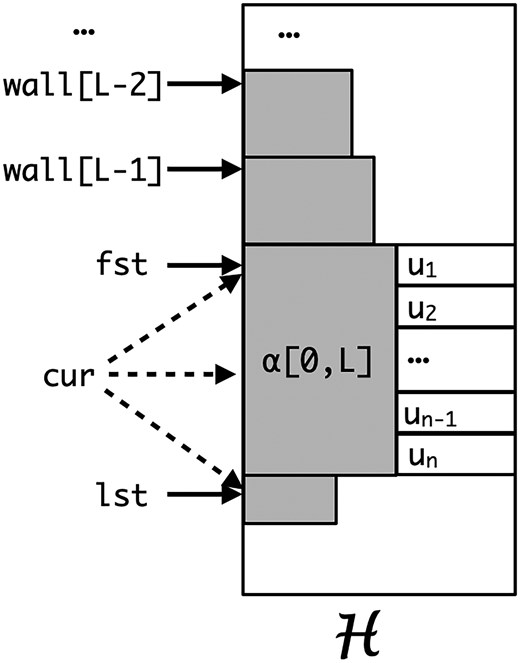
The problem is for each $K$-mer in the first index, say $\alpha = \mathcal{G}[i].kmer$ to find the range $[fst_i,lst_i)$ in the second index and length $L_i$ such that $lcp(\alpha, \mathcal{H}[j].kmer) = L_i$ for all $j \in [fst_i,lst_i)$, and $lcp(\alpha, \mathcal{H}[j].kmer) < L_i$ for all other $j$. Clearly, the adaptamers locate in positions $\bigcup_{j \in [fst_i,lst_i)} \mathcal{H}[j].loc$ in the second genomes.
The key logic is:

a) find $cur_i$ in $\mathcal{H}$ such that $\mathcal{H}[cur_i-1].kmer < \alpha \leq \mathcal{H}[cur_i].kmer$. It is clear the longest prefix match to $\alpha$ occur at either $cur_i$ or $cur_i-1$. Furthermore $cur_i$ must in the interval $[fst_i,lst_i]$, note that if $cur_i-1$ is the longest prefix match, $cur_i = lst_i$.

b) In $(fst_i,lst_i)$, we know the lcp of each element is $\geq L_i$. So we can use this information to extend $cur_i$ to $fst_i$ and $lst_i$ i.e. $fst_i = \max \{j \leq c \mid \mathcal{H}[j].lcp < L_i \}$ and $lst_i = \min \{j > c \mid \mathcal{H}[j].lcp < L_i \}$, where $c$ is any element in $[fst_i,lst_i)$.
In the algorithm, we seek to find $cur_i, fst_i ,lst_i$ and $L_i$ and maintain a $k$ elements vector $wall_i$ ($k < L_i$) such that $wall[k] = \min \{j \mid lcp(\alpha, \mathcal{H}[j].kmer) \geq k\}$ i.e. the upper boundary of each block of $lcp = k$. The algorithm does inductively, let’s assume we already know everything of $\alpha = \mathcal{G}[i-1].kmer$, seek answers for $\beta=\mathcal{G}[i].kmer$, and denote $\lambda = \mathcal{G}[i].lcp$. The algorithm can be split into two parts to explain a) split the cases and we can determine the answers directly without extra effort b) for complicated cases, we extend $cur_i$ to $fst_i$ and $lst_i$. I will explain it in the following subsections. The visualization of these concept see the below figure.

split cases

To make life easy, sometimes I use $L$ to represent $\alpha.L$.

If $\lambda > \alpha.L$, of course, $\beta$ cannot find a shorter prefix match than $\alpha.L$, because they share a prefix of length $\lambda > \alpha.L$. Can we find that a longer prefix match than $\alpha.L$ for $\beta$? If so, because $\alpha[0,\lambda] = \beta[0,\lambda]$, $\alpha$ could find a longer prefix match in $\mathcal{H}$. In this case, we just copy every answer of $\alpha$ to $\beta$.
If $\lambda = \alpha.L$ and $\alpha.cur = \alpha.lst$, we know immediately $\alpha$ shares a prefix with $\mathcal{H}[\alpha.cur-1].kmer$ of length $\alpha.L$ and the common prefix of $\mathcal{H}[\alpha.cur].kmer$ is smaller than $\alpha.L$ i.e. $\alpha[0,L] < \mathcal{H}[\alpha.cur].kmer[0,L] = \mathcal{H}[\alpha.lst].kmer[0,L]$. Recall that $\beta[0,L] = \alpha[0,L]$, so $\beta.L \geq \alpha.L$. Can we have longer match for $\beta$? No, $ \beta[0,L] = \alpha[0,L] < \mathcal{H}[\alpha.lst].kmer[0,L]$, so we will find a same slot for $\beta$ i.e. $\beta.cur = \alpha.cur$, $\beta$ cannot have longer match with both $\mathcal{H}[cur-1].kmer$ and $\mathcal{H}[\alpha.cur].kmer[0,L]$. In this case, every answer of $\alpha$ is same to $\beta$.
If $\lambda = \alpha.L$ and $\alpha.cur < \alpha.lst$, then a longer match of $\beta$ to $\mathcal{H}$ is possible. But it cannot happen with $\mathcal{H}[\alpha.cur-1].kmer$, i.e. we do not need to search upward. We will extend it from $\alpha.cur$ i.e. call extension procedure, the detail is described in next subsection.
If $\lambda < \alpha.L$, then $\beta[0,L] > \alpha[0,L]$ implying $\beta.cur \geq \alpha.lst$ (because all the entries in $[fst_i,lst_i)$ have a same prefix of length $\alpha.L$). And also $\beta$ will have a match with length $\geq \lambda$. So, we move forward from $\alpha.lst$ to search for $\beta.cur$. Note that, if the $j$th entry has prefix as $\alpha[0,\lambda+1]$, $\beta$ cannot have a longer match than $\lambda$ i.e. as long as $\mathcal{H}[j].lcp > \lambda$, we need to keep moving forward. When we stop moving i.e. $\mathcal{H}[j].lcp > \lambda$ does not hold, we have two situations

a) $\mathcal{H}[j].lcp < \lambda$, then $\beta[0,\lambda] = \alpha[0,\lambda] < \mathcal{H}[j].kmer[0,\lambda]$. That means we found $\beta.cur$ that is $j$, and $\beta.L = \lambda$, $\beta.lst = cur$. And $fst_i = \alpha.wall[\lambda]$, recall that $\alpha.wall[\lambda]$ upper boundary of the block with prefix $\alpha[0,\lambda]$. Furthermore, $\beta.wall$ can succeed all the elements of $\alpha.wall[0,\lambda]$.

b) $\mathcal{H}[j].lcp = \lambda$, then $\beta[0,\lambda] = \alpha[0,\lambda] = \mathcal{H}[j].kmer[0,\lambda]$. That means $\beta$ could have longer match, and then we will call extension procedure.

extension

In this subsection, we will talk about extension procedure that response the task of extending longer match (see the cases mentioned in the above subsection).


1
2
3
4
5
6
7
8
9
10
11
12
13
14
15
16
17
18
19
20
21
22
 Extension () {
	while (L < K) {
		while (H[cur].kmer[L+1] < \beta[L+1]) {
			cur +=1
			if H[cur].lcp < L then {
				lst = cur
				return
			}
		}
		if H[cur].kmer[L+1] > \beta[L+1] then {
			break
		}
		L += 1
		fst = wall[L] = cur
	}
	lst = cur + 1
	if L < K then {
		while H[lst].lcp >= L and lst <= fst + \tau do {
			lst += 1
		}
	}
}

First our big goal is to move forward to find $\beta.cur$ until $\mathcal{H}[\beta.cur].kmer \geq \beta$. So, we move each 2-bits (a base) i.e. L in big while-loop and move each entry i.e. cur in the small while-loop.
In the small-loop, when we met $\mathcal{H}[cur].lcp < L$, we know we found our $\beta.cur$, and then $\beta.L$ is the current L, $\beta.lst = \beta.cur$.
When we exit the small while-loop, i.e. $\mathcal{H}[cur].kmer[L+1] \geq \beta[L+1]$

a) $\mathcal{H}[cur].kmer[L+1] > \beta[L+1]$, we found the current $cur$ is $\beta.cur$ and then we break the big while-loop. Then we know $\beta.L$ is the current L and $\mathcal{H}[cur].kmer[L] = \beta[L]$, then $lst > cur$ and we need start $lst$ from $cur+1$ and move forward. When we find $\mathcal{H}[cur].lcp < L$ or the number of adaptamers is greater than $\tau$, we will stop.

b) $\mathcal{H}[cur].kmer[L+1] = \beta[L+1]$, we know the length of common prefix is at least $L+1$, and we will start next round. In this case, we will update $wall[L+1] = cur$ that is the upper boundary of block with prefix $\beta[0,L+1]$, and we can update fst=cur (if $\beta.L$ is L+1, then fst is correct, that is also the reason when we exit the big loop or return, we do not need to update fst again).
Another case is $L=k$, in this case we update $lst = cur +1$ is enough. Of course we can move forward to find the correct $\beta.lst$, but we can leave it and then looking for positions in $\bigcup_{j \in [fst_i,lst_i)} \mathcal{H}[j].loc$ (hence, we do not need to find the final $lst$, when we looking for location of $\beta$ in $\mathcal{H}$, it achieves the same results). Sure, we only report the adaptamers with $\leq \tau$ copies.

concern

Call back the the definition of adaptamer, they are not symmetrical. FastGA provides -S option to find adaptamers by running the merge of $G$ versus $H$ and then of $H$ versus $G$ and taking union. They anecdotally observe that the difference is primarily that FastGA finds additional short repetitive alignments in $H$. Their advice is if you are not interested in the repetitive matches between non-homologous regions, we can just do one side alignment.

Find Seed Chains and Alignment

After finding the adaptamers, now we move to the seed chain and alignment part. For each adaptamer pair, we denote it as a triple $(i,j,t)$, where $i$ and $j$ are the starting positions of genomes $G,H$ (in reality, it contains two parts, i.e. contig numbers and positions $p$ ) and $t$ is the match length. For each adaptamer pair, the adaptamer in the first index is always in the forward orientation so that redundant hits in which both seeds are in the opposite orientation are not considered. For the chain of seed, FastGA is seeking

Adaptamer seed hits lie in a narrow diagonal band of width, say $D$ (default as $64$);
Any pair of consecutive seeds on the chain are not further apart than $A$ (default as 1000) anti-diagonals.

To find the chain efficiently, FastGA creates a list of records $(c_i,c_j,b,a,r,t)$, where

$c_i,c_j$ are the contig numbers, $p_i,p_j$ are the positons
$b= \lfloor (p_i-p_j) / D \rfloor, b \in [-\vert c_j \vert /D , \vert c_i \vert /D]$. In other words, we split the dynamic graph into several band of width $D$.
$a = p_i +p_j$ is the anti-diagonal for the pair
$r = (p_i-p_j) \mod D$ use to recover $p_i,p_j$ i.e. $p_i = (a + (Db +r))/2$ and $p_j = (a - (Db+r))/2$
$t$ is also the match length

Then we find we can easily found chains by sort the above sextuplets by their first four components.

All the seed hits between a pair of contigs and are grouped together in the sorted list.
The seeds in each diagonal band are consecutive and in order of their anti-diagonal within the band
We can easily determine if two consecutive seed hits are separated by more than $A$ anti-diagonals in linear time.

However, we are looking for the chain within any band of width $D$. To do so, we can merge the adjacent bands. This could introduce the seed hits with width up to $2D$. We can filter them carefully, but FastGA choose to keep it and this issue will be addressed in the following alignment step (slightly influence the search time in the alignment). FastGA tries to passes through the tube of each chain. The tube is the rectangular region of the d.p. matrix that is bounded by the lowest and highest diagonals, $d_{low}$ and $d_{high}$⁠, among the seeds in the chain, and the lowest and highest anti-diagonals, $a_{low}$ and $a_{high}$⁠, where both ends of the seed hits are considered.

FastGA uses the very rapid wave-based algorithm for finding local alignments, called LA-finder. Note, given an anti-diagonal and $d_{low}$ and $d_{high}$⁠, LA-finder finds the best local alignment that passes through the anti-diagonal between the diagonal bounds.

For each chain’s tube, LA-finder is called on the anti-diagonal $a_{low} + 2D$⁠, or ($(a_{low} + a_{high})/2$) if $a_{low} + D \geq a_{high}$.
If the alignment returned is sufficiently long and sufficiently similar (both parameters that can be set by the user), then the alignment is collected for possible output.
We denote anti-diagonal of end of the returned alignment as $a_{top}$.
If $a_{top} \geq a_{high}$ then the tube is considered processed, otherwise we set $a_{low}$ as $a_{top}$, and search the truncated tube is again.
For each pair of contigs, FastGA removes all the redundant alignments. The bounding box of an alignment is the smallest rectangle that contains all the points on the alignment path. We consider an alignment to be redundant if it is entirely within the bounding box of another alignment.

Storing and Delivering Alignments

Trace Points

Suppose we have an alignment that aligns $A[ab,ae]$ against $B[bb,be]$, we denote $n = ae - ab$, $d$ as edit distance and $\epsilon = d / n$ as sequence dissimilarity then we know $be - bb \leq n(1 + \epsilon) = O(n)$. There are two obvious approaches:

just record 4 interval endpoints and recompute the detail when needed, we need $O(1)$ space to store but $O(n+d^2)$ expected time to deliver ($O(nd)$ for the worst case, see Myers-Ukkonen wave algorithm).
record all the details but delivered in linear time e.g. CIGAR string. We require $O(d)$ space (only storing the edit operations and corresponding positions) for storage and $O(n)$ to deliver the alignment.

Note the product of work and space are $O(nd)$ in both cases.

To have a continuum of space-time trade-offs between the two methods, FastGA use the idea of trace points. The intuition behind this idea is we split the alignment into small panels with length $\delta$ and reconstruct the alignments of each panels.

Formally, we split $A[ab,ae]$ into $A[ab,x_1\delta], A[x_1\delta, x_2 \delta], \cdots A[x_t\delta,ae]$, where $x_1 = \lfloor ab/\delta +1 \rfloor, x_i = x_{i-1}+1$ and $x_t = \lfloor (ae - 1) /\delta \rfloor$. In fact, we do not need to store these middle points, if we know $\delta$, the division of $[ab,ae]$ is determined. Next, based on the above devision, $B[bb,be]$ can also be partitioned into corresponding panels, say $B[y_0,y_1],B[y_1,y_2],\cdots, B[y_t, y_{t+1}]$, where $y_0 = bb, y_{t+1}=be$. But, note here, the partitioning may not be unique (because the inserted symbols in $B$ can be split by any position). But we can place all the inserted symbols of $B$ into the left interval (see the below figure).

Denote $b_i = y_{i+1} - y_i$, we know $\delta (1- \epsilon ) \leq b_i \leq \delta(1+\epsilon)$. And then we have the trace point array $<b_0,b_1,\cdots,b_t>$, and we only need to store these $t+1$ elements and four endpoints for the alignment. Given the array, we can easily reconstruct $x_i$ and $y_i$ in $O(n / \delta)$ time. We will analysis the theoretical running time for delivering the $t+1$ subalignments for $A[x_i \delta,x_{i+1}\delta]$ versus $B[y_i,y_{i+1}]$.

The below analysis based on a theoretical results from “skewed-wave” algorithm. The running time is $O((n+m)(d-\vert n-m\vert +1))$, where $d$ is the number of differences.
Suppose $b_i = \delta + x, x > 0$, and we use $d_i$ to denote the number of differences for subproblem $i$. Hence the running time for each subproblem is
\[\begin{align*} O((\delta + b_i )(d_i - \vert \delta - b_i \vert +1)) &= O((2\delta + x)(d_i - x +1))\\ & = O((2\delta + x) + (2\delta + x)(d_i - x))\\ &= O(\delta + (\delta + x)(d_i - x)) \\ & = O(\delta + \delta d_i + x((d_i-x)-\delta)) \\ & \leq O(\delta + \delta d_i + x((b_i-x)-\delta)) \\ & = O(\delta (d_i +1)) \end{align*}\]
If $b_i = \delta - x$, then it takes $O(\delta (d_i - (\delta -x))) = O(\delta d_i)$. Then we know the total running time is $O(\sum_i \delta (d_i + 1) = O(n + \delta d))$.

In FastGA, they use $\delta = 100$ to make $b_i$ fit into a byte (for large insertions, $b_i$ could exceed $255$, but such large gap are not allowed in FastGA). In empirical trails, FastGA convert trace-point encoded ALN files to PAF format with CIGAR strings at a rate of roughly 100 million aligned bases per second on a laptop.

When FastGA deliver the alignment, actually we have a chance to refine the gaps. Because, we can have less gaps with same optimal edit distance, which can correct many alignment.

FastGA -- fast genome alignment